C-State
C-State

Home


Motivation


C-State (Chromatin-State) was conceived to address the needs of a growing user base in our lab that works with large NGS datasets. Despite the existence of several tools for epigenetic analysis, identification of common epigenetic patterns and their visualization across gene subsets in the context of expression profiles remains a difficult task for biologists. C-State is an interactive platform that enables experimentalists who lack bioinformatics support to investigate epigenetic landscapes across multiple datasets for comparative epigenomic analysis.

The first version of C-State (v0.1) was released in April, 2016. Several new features have since been added based on user inputs. You can use the "Launch C-State" button on the right to open the latest stable version (0.2.3) or you can try the development version (0.2.4-dev). The source code of C-State is available at our GitHub page under an MIT license.


Current version: 0.2.3

OS: Windows, MacOS, Linux

Browsers: Tested on Chrome, Firefox, and Edge


Key features


C-State identifies epigenetic patterns across genomic regions and filters genes based on their chromatin signatures. It takes advantage of the “small multiples” paradigm (Tufte, 1990) to facilitate simultaneous visualization and comparison of epigenetic marks on genes in the context of their expression profiles. C-State follows an MVVM (Model-View-View Model) architecture, and is written in JavaScript (ES2015) using VueJS (View layer) and d3.js (plotting). Its features include:


What you can do with C-State (see Use Cases)


C-State is an integrated visualization platform that enables automatic retrieval, processing and querying of data from whole genome experiments (ChIP-chip, ChIP-Seq, microarray, and RNA-Seq). Using C-State, it becomes easy for bench biologists to accomplish the following tasks without resorting to command-line tools:


Tutorial


Video Demos


Launching C-State and Uploading Data Files

Filtering Data


Epigenetic Pattern Search Using Filters

Downstream Plots and Tables


Data Input: Files accordion


C-State Main View
Main View of C-State showing expanded Files accordion. Load a list of genes as described below in this tutorial or click on "Load Example Data" for analyzing up to 6 pre-loaded datasets.

Load a list of target genes

  1. Create a list of target genes to be analyzed as a simple text file containing gene identifiers (Official Gene Symbols or other IDs) - one entry per line, see sample txt file.

  2. Load the gene list txt file via the “Load gene list/C-State data” button. Choose the species and genome build from the dropdowns provided.

  3. The loaded file is indicated. Select the appropriate File Type, Gene identifier and regions around the genes to be included as upstream and downstream flanks. This is set to 20KB on either side of the gene body by default.

    C-State automatically extracts data for the target genes in the list, along with the chosen flanks, from whole genome ChIP-seq / ChIP-chip datasets (see steps 4 and 5).

    Note: If you have used C-State before and want to re-analyze your data, you can directly load the previously saved C-State JSON file instead of the gene list and select “Previous Plot Data” as the File Type.
  4. C-State Tutorial 1
    Gene list (human_330_genes.txt) loaded into C-State


Load whole genome datasets

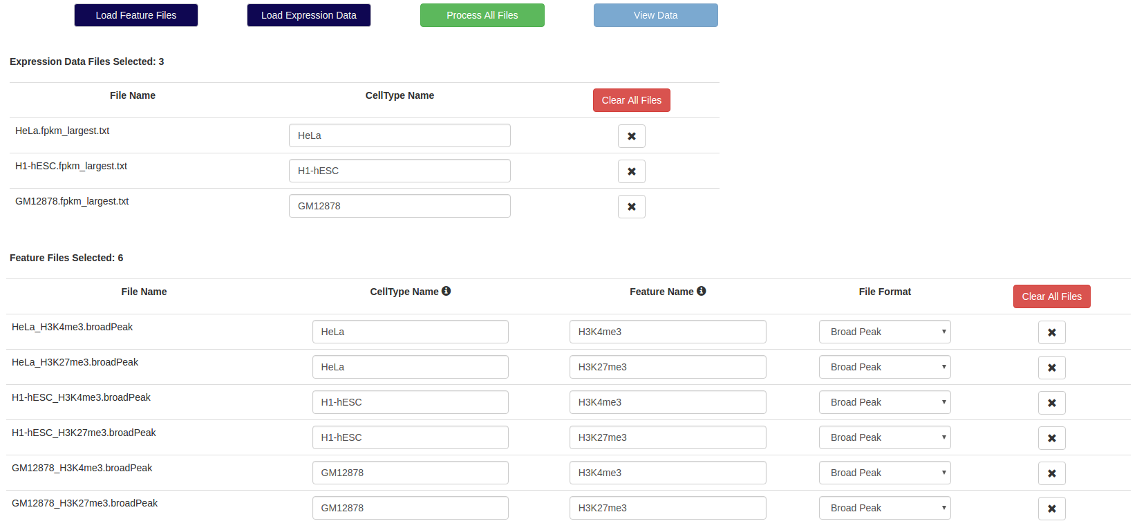
  1. Options to load the whole genome peaks/feature files now appear. These are raw data files from the user’s experiment or from other studies such as ChIP-seq for histone marks and transcription factors that provide peak coordinate details in BED format. They can be named in the format CellType_Feature (for eg, H1hesc_H3K4me3.broadPeak; see sample format) and directly loaded via the “Load Feature Files” button. The auto-filled file details based on the file name appear below; these can be edited or entered manually as well.
    File formats supported by C-State...

    C-State currently supports feature information in BED and BED-like formats such as broadPeak and narrowPeak. For a detailed description of these file formats, please see this page.


  2. If gene expression data of corresponding cell types is available, it can be loaded via the "Load Expression Data" button (see sample format).

  3. Click on the “Process All Files” button. C-State extracts the relevant gene information for all target genes from the genome file, and validates the format of feature files and expression data files. Troubleshooting tip: C-State indicates if any genes could not be mapped. In case of an error in the file format, no gene will be mapped and C-State will alert the same.

  4. Click on “View Data” to open the View accordion. This displays gene-specific feature plots of all the target genes and their flanking regions across the specified cell types.
    How C-State maps features to gene panels…

    1. Relevant gene information such as its genomic coordinates, strand, number of exons etc. are retrieved from the genome file
    2. Features mapping to any of the target genes and their flanks are retrieved from each of the feature files
    3. Feature coordinates are converted relative to the transcription start site (TSS) of each gene they map to
    4. Gene expression values for the target gene are retrieved from each of the cell type-specific expression data files
    5. All the peak features and genes are then corrected for gene orientation (strand), and plotted with respect to the TSS,such that all genes are oriented similarly irrespective of their strand-of-origin (upstream region to the left and downstream to the right of the TSS). This gene-centric format allows for easy visualization and comparison of trends across genes and locations


  5. C-State Tutorial 2
    Features datasets loaded into C-State


Data Visualization: View accordion


The View accordion opens to display feature plots for all the genes of interest across the loaded cell types.

C-State Tutorial 3
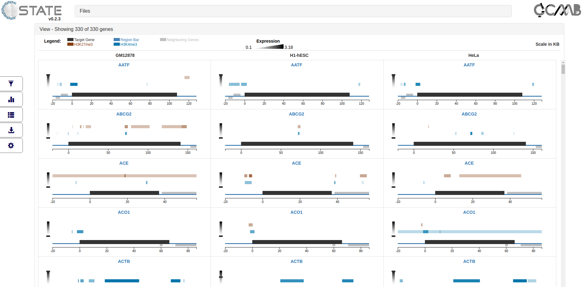
Main view of C-State showing expanded View accordion. Compare epigenetic features here or use the control panel on the left to access additional functionality, as described in subsequent sections.


Main view

How C-State displays gene panels…

C-State uses the small multiples paradigm to render simultaneous plots for comparison. The default grid view is organized for simultaneous depiction of all peak features at the target loci across multiple cell types; data panels are arranged column-wise and each gene is displayed side by side across all samples, facilitating comparative visualization. C-State uses dynamic width for plots and adapts to the number of cell types / conditions specified so that the plots are not rendered off-screen. Scrolling through the grid layout (drag scroll enabled) allows rapid browsing through all the genes of interest.


  1. The View accordion is populated with gene-specific data panels, arranged based on the number of conditions loaded. The number of genes displayed, active filters (if any filters are applied) and feature cut-offs (if applied) are indicated on the right side of the header bar. A legend (created based on the names of the Features Files and the range of gene expression values) is displayed at the top left. Note: Feature cut-offs (based on peak size and score) and gene expression range can be set from the Settings panel.

  2. The region of interest is indicated by a scaled blue line with the target gene (indicated by its panel header) shown as a black bar on it. Neighboring genes are indicated as silver bars and plotted either above (indicating the same strand as target gene) or below (opposite strand) the region bar; mouse hover displays gene name and size. Note: Attributes such as target gene exons and neighbors display, color scheme of features, bar colors and heights can be changed in the Settings panel.

  3. The scale is in KB and specific to each gene in order to maintain visual similarity across all the genes, irrespective of size. Orientation of each gene is taken into account, and all features are corrected and plotted with respect to the TSS (upstream region to the left and downstream to the right of the TSS for all panels).

  4. Features from the raw peak data files are calculated with respect to TSS, corrected for orientation and plotted as shaded bars on multiple tracks above the gene; the opacity of the bars is a function of the peak intensity scores, which are displayed on mouse hover. Note: Color scheme and bar heights can be changed in the Settings panel. Quality of peaks to be displayed (based on intensity score and/or size) can be also be set.

  5. Cell type specific gene expression value is indicated as a notch on a heatmap slider on the left of each panel

  6. All the gene panels in the main view can be saved as an svg image using the Downloads button in the control panel on the left (4th button).

Gene Modal

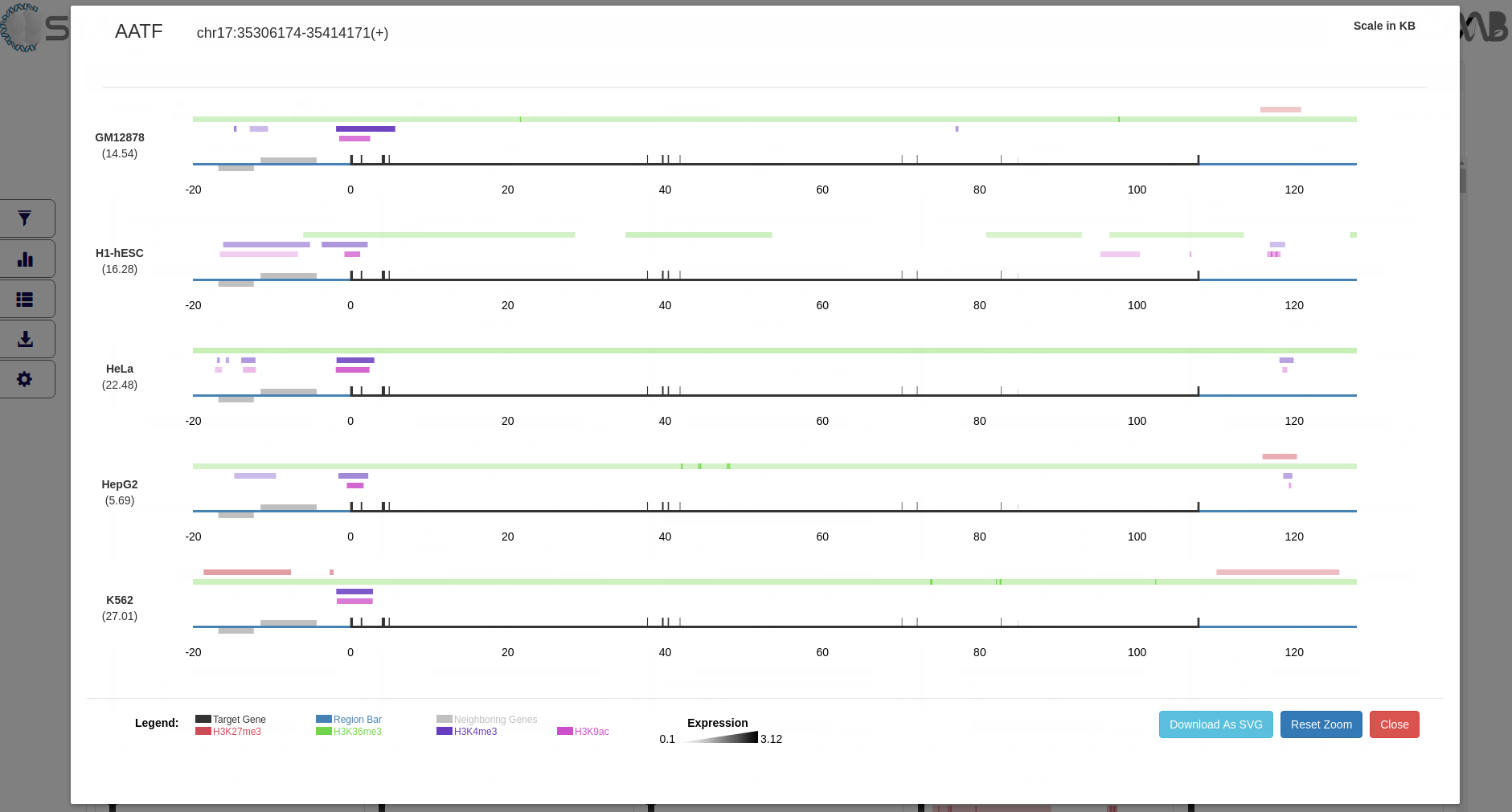
  1. Clicking on a gene name from the grid panels opens its modal, where the data representing the gene in multiple cell-types is stacked vertically for closer inspection. The expanded modal view provides a gene-specific view across cell types and features by utilizing the larger aspect ratio of a landscape layout. Target gene exons are displayed as black boxes on the gene body. Note: Exon display can be toggled both in the main and modal views from the Settings panel.

  2. The modal view is interactive and supports panning and interactive zoom control; the zoom is linked to all the data tracks for seamless comparison, and can be reset to the original state with the “Reset zoom” button. Feature (peak) and gene information is revealed on mouse-hover. Note: Feature attributes (color, bar height) can be changed for the modal in the Settings panel, independently or linked to main view.

  3. Context specific information (genomic coordinates and orientation) is indicated on the top left. Gene expression value is mentioned in parentheses under the name of each cell type. Legend is displayed on bottom left. The modal view can be saved as an svg image using the "Download as SVG" button.

  4. C-State Tutorial 4
    Gene Modal view


Data Analysis and Output


5 buttons on the left side of the Files and View accordions provide access to other functionalities of C-State.

Filters Panel - Search for Epigenetic Patterns

One of the novel advantages of C-State is that it enables filtering and searching for cell type specific epigenetic features and patterns. This is particularly useful for biologists to identify gene or cell type specific epigenetic patterns without any need for programming or bioinformatics.

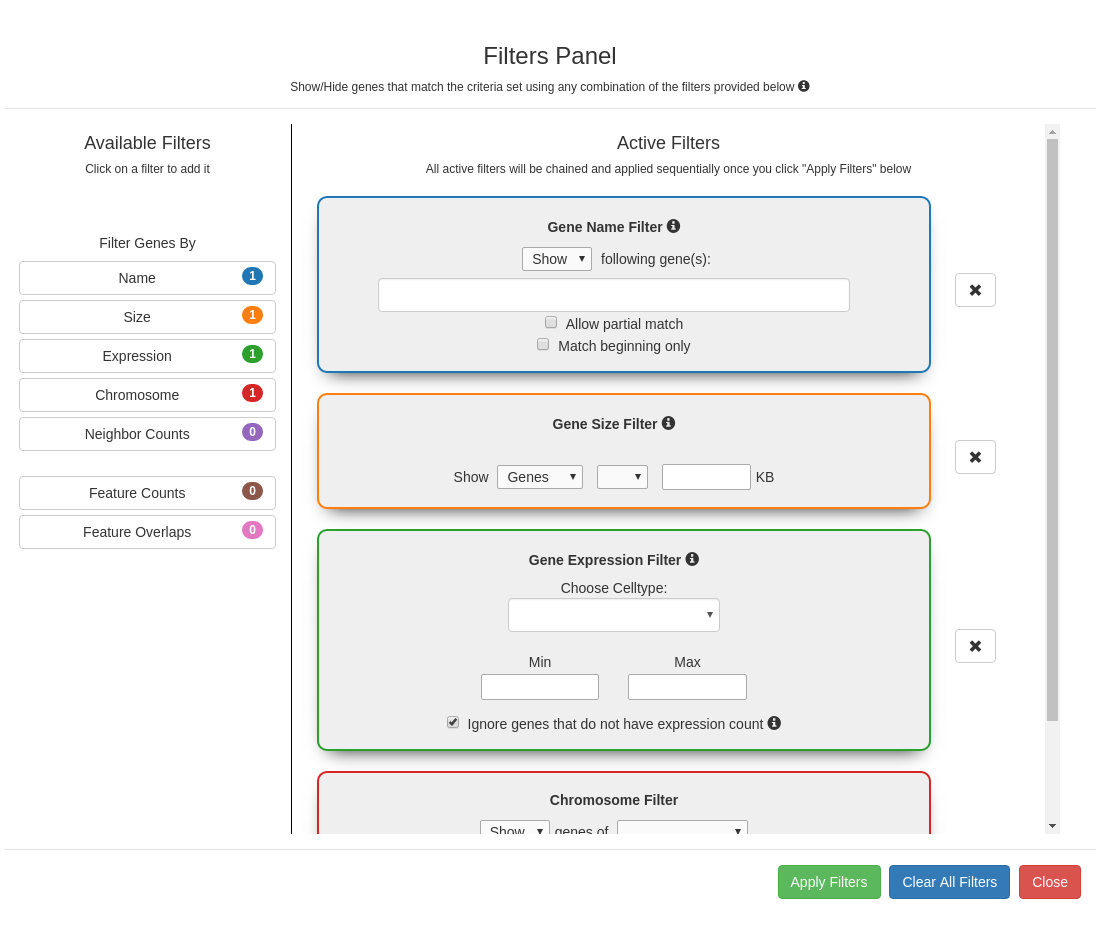
The filters module (1st button in the control panel) allows the user to search for genes containing specified patterns of genomic and/or epigenetic features. Options in the filters appear automatically in the drop down menus based on the raw data files provided to C-State. The filters can be chained together in the order of their selection to build complex user-defined pattern searches since each output gets applied to the successive filters in the chain on clicking the “Apply Filters” button (see use case examples).

Gene Name Filter

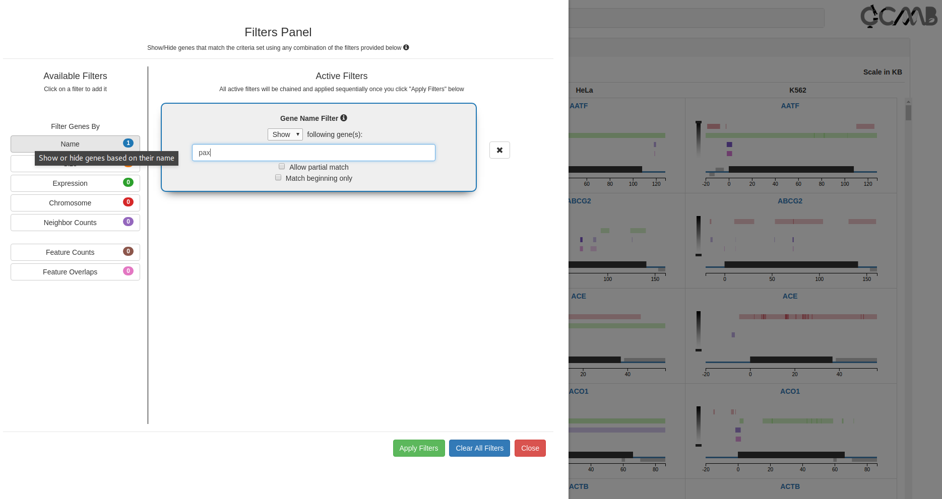
Search for a gene by name or ID; a set of gene names can be also be pasted to display all the genes that match the given name(s). Ticking the 'Allow partial match’ or 'Match beginning only' checkboxes allows the user to filter for all the genes which have similar names (eg., gene families such as Hox, PAX etc).

Gene Size Filter

Specify size cutoffs for genes or the total regions (including flanks) using a range of operators provided in the drop down.

Gene Expression Filter

Search for genes/transcripts that fall within a given expression range in a cell type.

Chromosome Filter

Show or hide genes belonging to a particular chromosome. Chaining multiple chromosome filters allows viewing genes across any chromosome combinations or across all chromosomes. This filter can also be used to display precise co-ordinates of a locus.

Neighbor Counts Filter

Search for genes according to the presence of neighboring genes around them using a range of operators. User can optionally choose to ignore or filter the dataset based on presence of other genes overlapping the target genes.


Apart from the above genomic filters that search based on gene size, location or genomic context, C-State also provides options to identify genes based on their epigenetic patterns.

Feature Counts Filter

Select from a set of operators to find genes that carry the desired number of cell type specific marks. The search can be further refined by specifying the distance of the marks from the TSS.

Feature Overlaps Filter

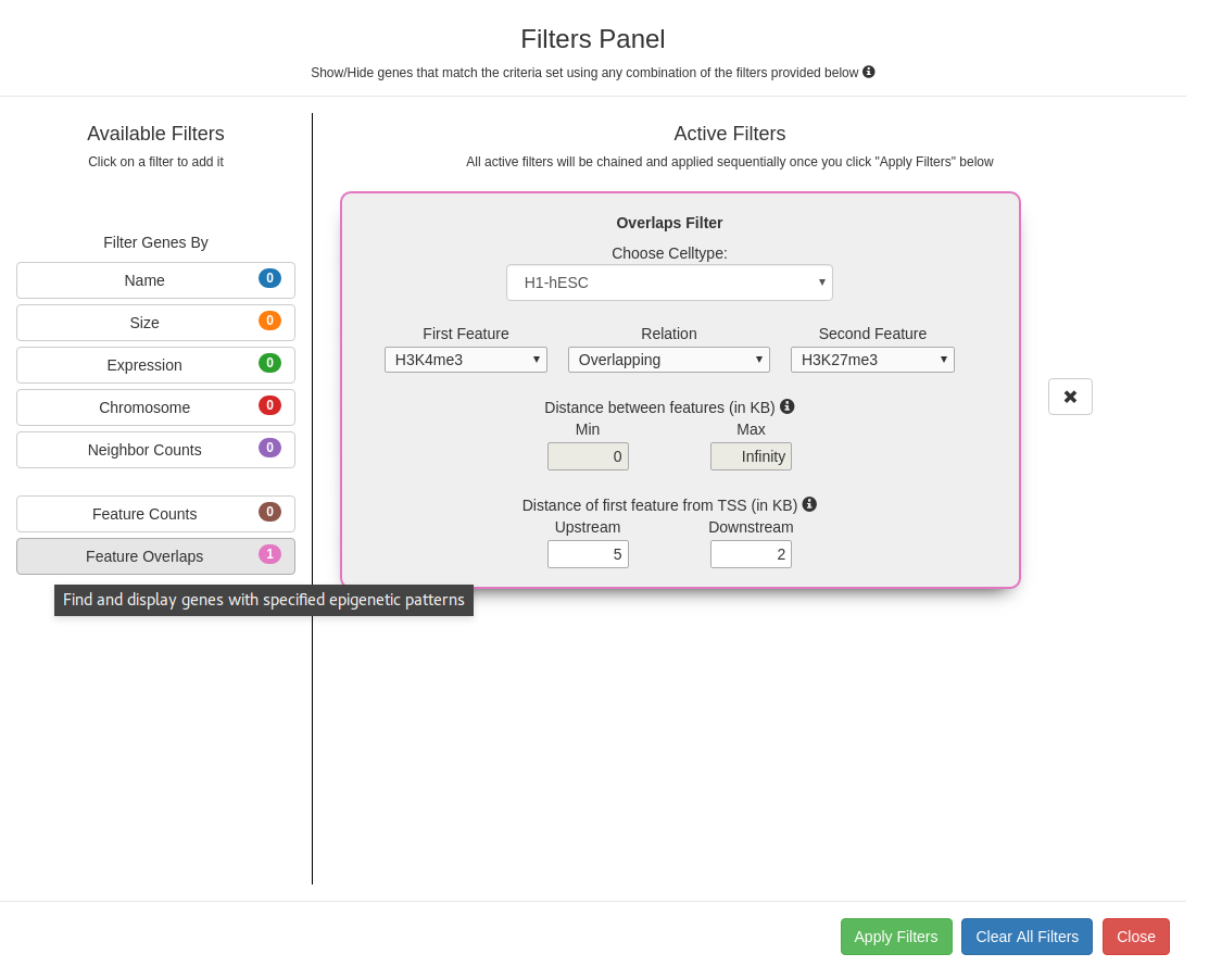
Filter to display genes based on cell type specific patterns of epigenetic marks. Select the two features that are to be viewed in the context of each other from the two drop-down menus and define their relationship using the relation dropdown:

  • Upstream To - The first feature is present upstream to the second feature
  • Downstream To - The first feature is present downstream to the second feature
  • Near - The first feature can be either upstream or downstream to the second feature
  • Overlapping - The first feature overlaps the second feature

The distance allowed between the two marks can also be specified; in case of overlaps, the min and max distance allowed between the two marks is 0 and this option gets disabled. The search can be further refined by specifying the distance of the pattern from the TSS.
C-State Tutorial 5
Filters panel showing the 7 available filters (Gene expression, genomic, and pattern filters). Clicking on a filter opens it in the Active Filters area for setting parameters. Successive filters get chained sequentially; clicking on the x next to a filter removes it from the chain. The filter combination is applied only on clicking the "Apply filters" button.

Once the filters are applied using the "Apply Filters" button, the filter panel slides back. The number of active filters are indicated in the header of the View accordion. Filtered output can be exported and saved.


Plots and analysis panel - Identifying Data trends


In addition to gene centric plots for visualization, C-State also allows users to identify cell type specific global trends in their dataset using the Plots and Analysis button (2nd button in the control panel). If filters are activated (from the previous panel), the plots can be generated only on the filtered gene subsets thus enabling a platform to analyze multiple specific versus global patterns.


Histograms

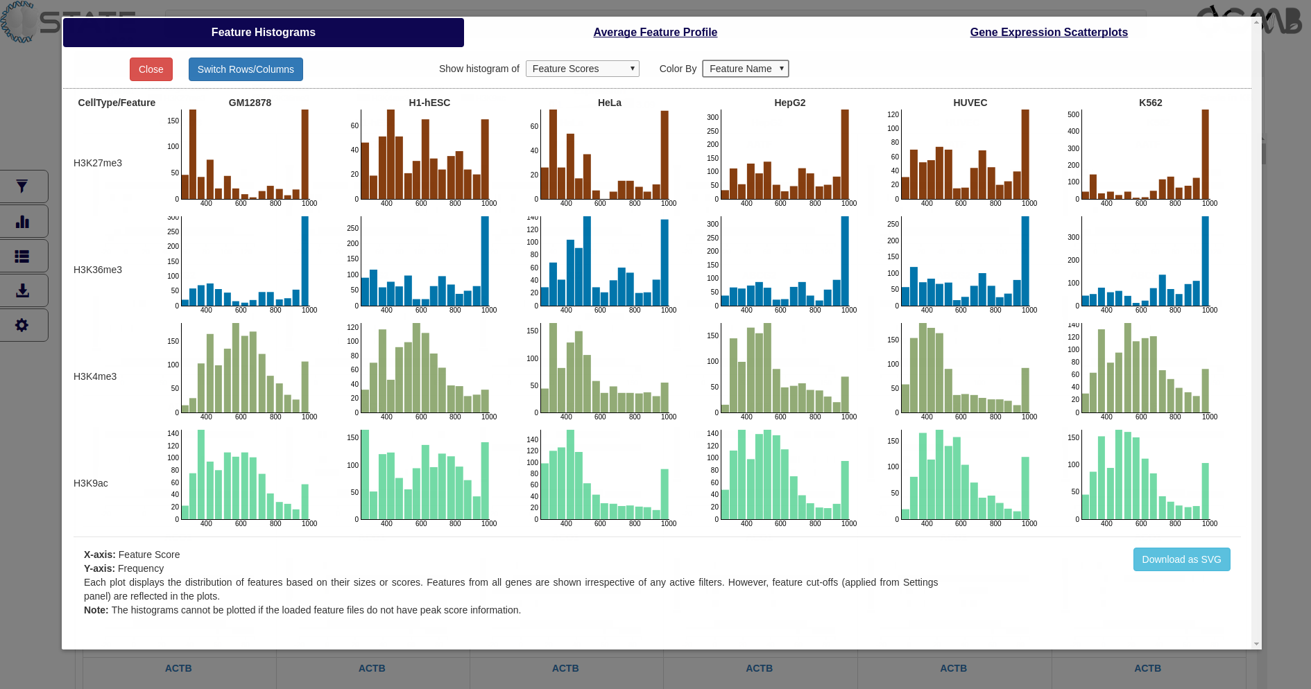
Display the frequency of features based on their size or score (X-axis) across all marks and cell types (arranged row- and column-wise respectively by default). Use the "Switch Rows/Columns" button to toggle the arrangement of cell types and features.

How histograms are generated...

If "Features Scores" is chosen in the dropdown menu and cell types are arranged column-wise:

  1. C-State retrieves the scores of all features in a given cell type
  2. The minimum and maximum scores of each cell type are calculated, so that the histogram bins are constant across multiple features
  3. The scores are separated feature-wise, and supplied to d3.histogram with the previously calculated minimum and maximum values as data range
  4. Score are divided into 20 bins, and the frequency of a given feature in each bin is plotted as a bar

If rows and columns are switched, the same steps are followed, except that the minimum and maximum values are calculated using the info of respective features across all cell types.

C-State Tutorial 6
Plots and Analysis panel (Feature Histograms) showing frequency of features based on their scores (peak intensity) and colored by feature name


Average Feature Profile

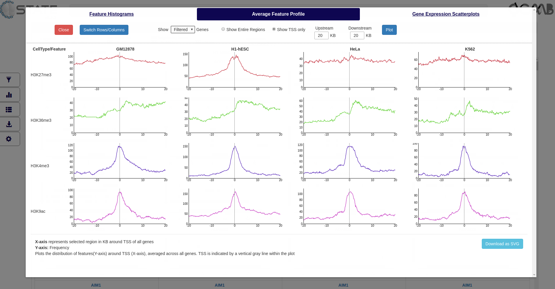
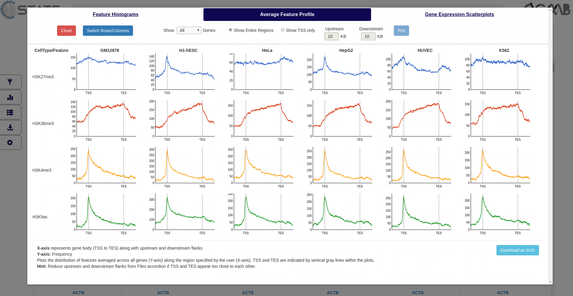
Plot the distribution of features averaged across all genes (Y-axis) along the region specified by the user (X-axis). The gene start and end positions and the chosen upstream and downstream flank sizes are indicated. Data can be plotted for a filtered subset (if any filters are activated) or for the entire list of genes and the Y-axis scale can be adjusted from the dropdowns above the plots.

How average profiles are calculated...

All genes and their respective flanks are divided into equal number of bins as follows:

  1. The number of gene body bins is determined by the median gene size in the list of target genes using a bin size of 100bp. For example, if the median size is 50KB, the number of gene bins is 500
  2. Upstream and downstream flanks are divided into 100bp bins
  3. Starting from the most upstream bin, C-State counts the features falling in each bin for all genes
  4. The frequency in each bin is plotted on Y-axis whereas the bins are represented on the X-axis
In case of TSS plots, upstream and downstream regions of TSS entered by the user are divided into 100bp bins instead of using median gene size.

C-State Tutorial 7
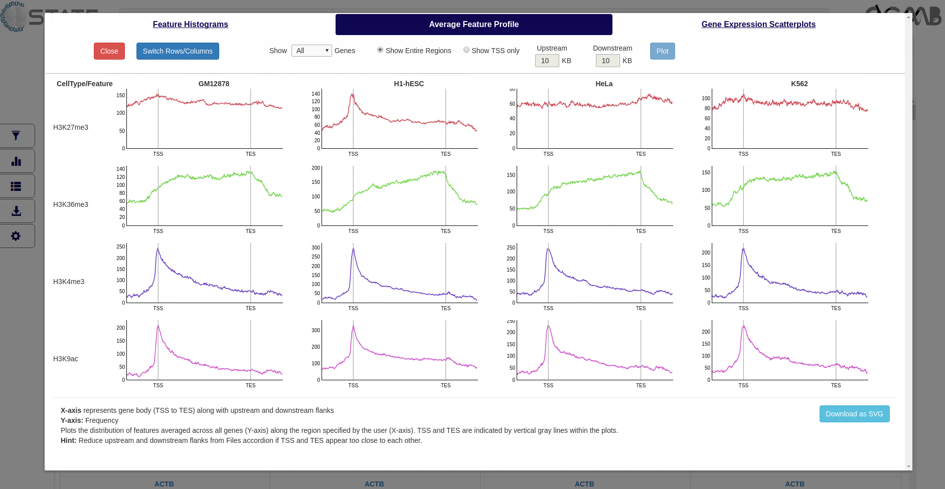
Plots and Analysis panel (Average Feature Profile) showing the average distribution of each mark with respect to the gene bodies (TSS to TES) along with flanking regions selected in the Files accordion


Gene Expression Scatterplots

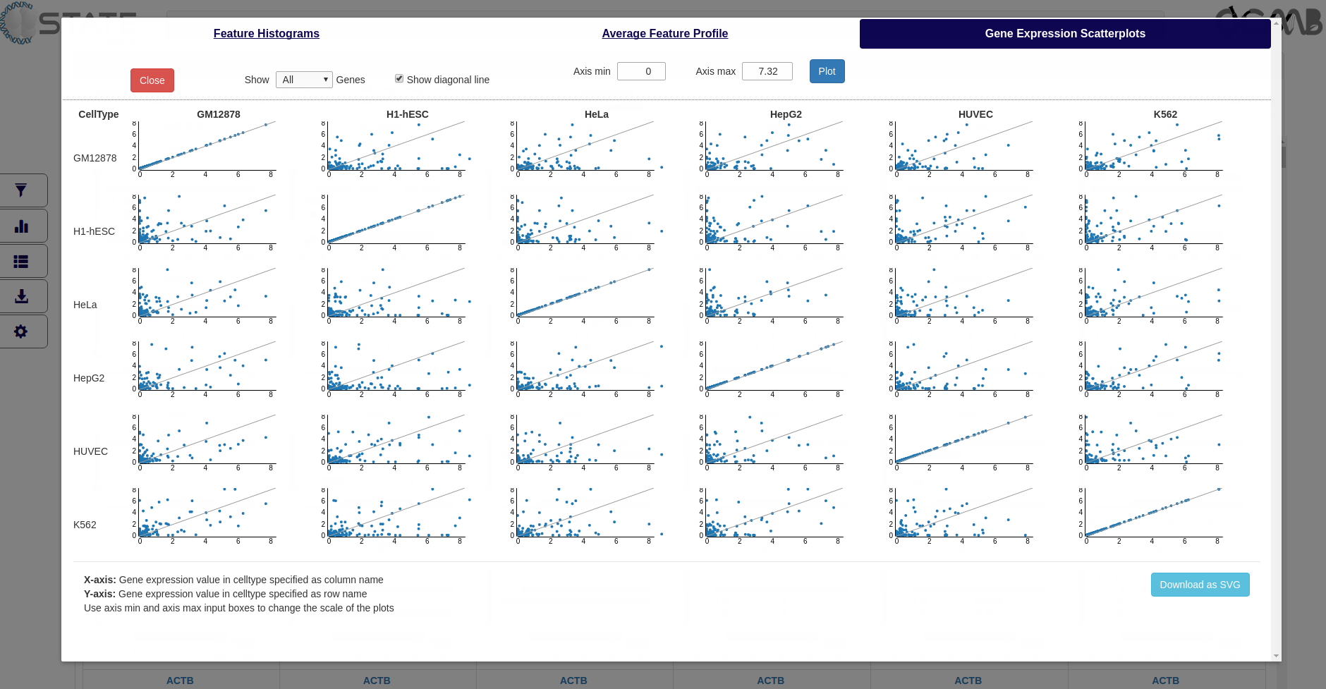
Plot the relative gene expression values between pairs of cell types. Expression level of a gene in the first cell type (column name) is plotted on X-axis, and its expression in the second cell type (row name) is plotted on Y-axis.

How gene expression range is determined...
  1. C-State calculates the cumulative minimum, maximum, and the 5th, 95th, and 99th percentile of expression values from the expression data files of all the cell types
  2. By default, the axis minimum and maximum are determined by the minimum and 99th percentile of the loaded datasets
  3. These values can be changed using the axis input boxes on the top of the plots

C-State Tutorial 8
Plots and Analysis panel (Gene Expression Scatterplots) showing comparative distribution of gene expression profiles for all target genes


Tables panel - View tabular data


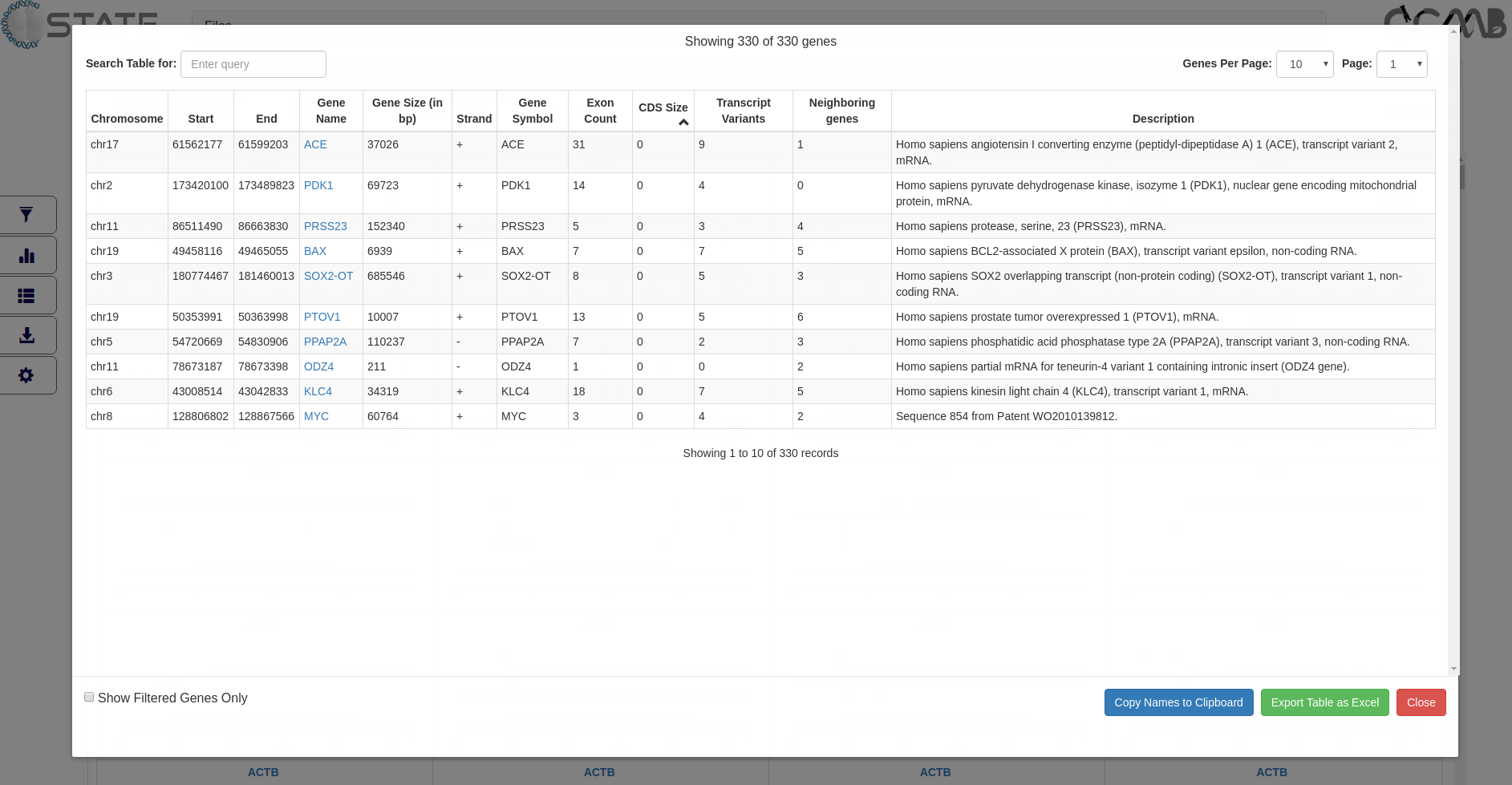
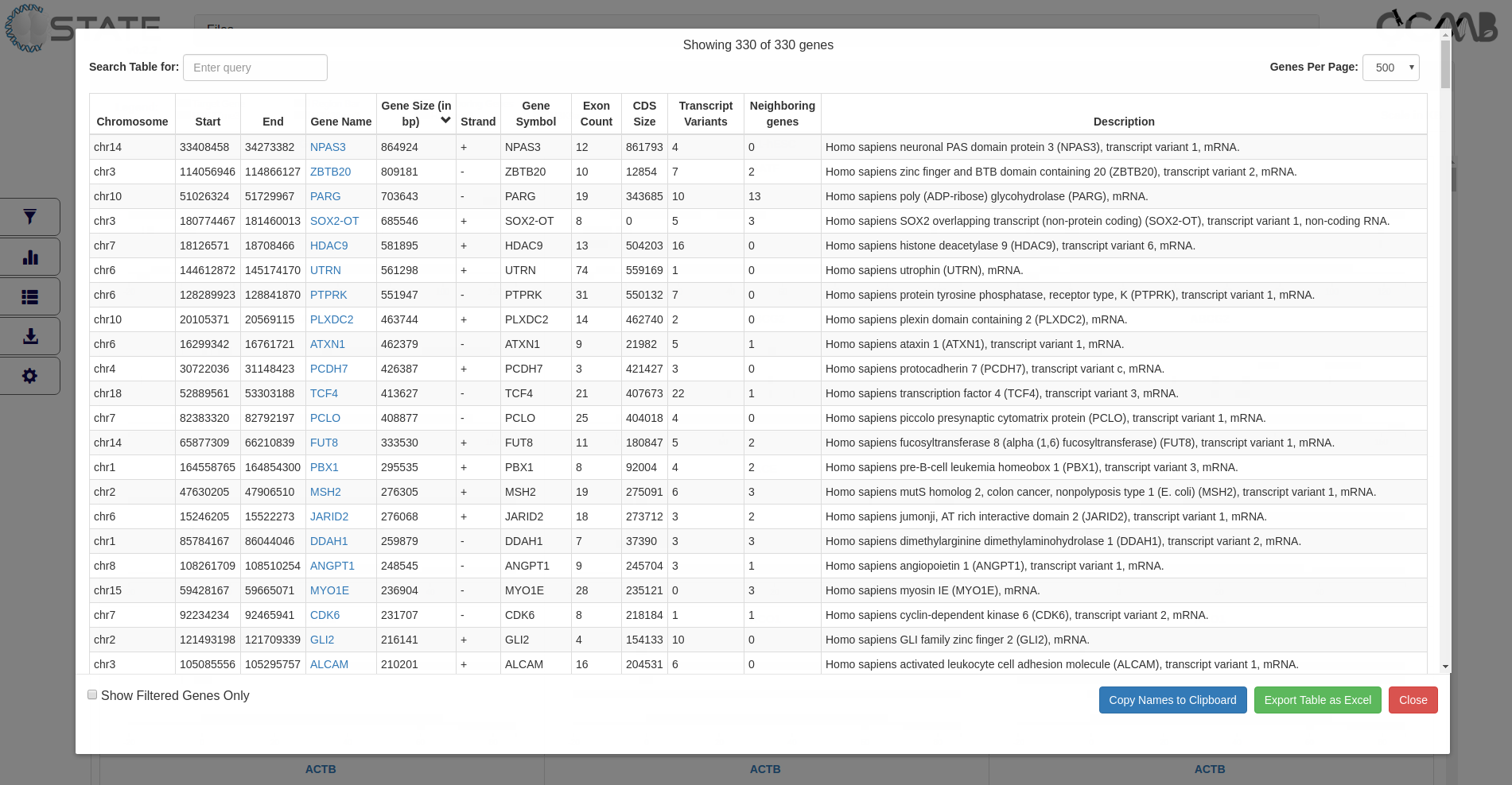
Tabular information (3rd button in the control panel) of the gene set is provided to display gene information of all or filtered subsets of genes (if filters are activated). The table is interactive and can be sorted on any of the columns. Clicking on the gene name opens the gene modal view for that gene. This feature is useful for sorting information based on user-defined criteria and subsequently viewing the gene panels in the desired order.
C-State Tutorial 9
Tables panel showing tabulated gene information of all target genes

The entries can be searched based on terms in any of the columns and arranged page wise using the controls at the top of the table. Clicking the “Copy to clipboard” option copies all the gene names displayed in the table for handy pasting into any other application or relevant rows may directly be copied from the table. Selected pages or the entire table can be exported and saved.


Downloads panel - Download Results

The Downloads button (4th button in the control panel) provides 3 options to save and export the various outputs generated in C-State.

C-State Tutorial 10
Downloads panel showing options to download multiple C-State outputs

Export C-State Summary - Export a txt file containing summary of the gene names, feature track settings, and active filters (if any).

Download View panels as SVG - Download all the gene panels in the View accordion as a single SVG file.

Download C-State JSON File - Download the entire session info and plot data as a JSON file. This file can be uploaded as "Previous C-State Data" from the Files accordion.


Settings panel - Change global settings


Settings changed from this panel apply across C-State, for visualization, filtering, plotting and analysis and also get saved in any exported / downloaded files.


Feature Tracks

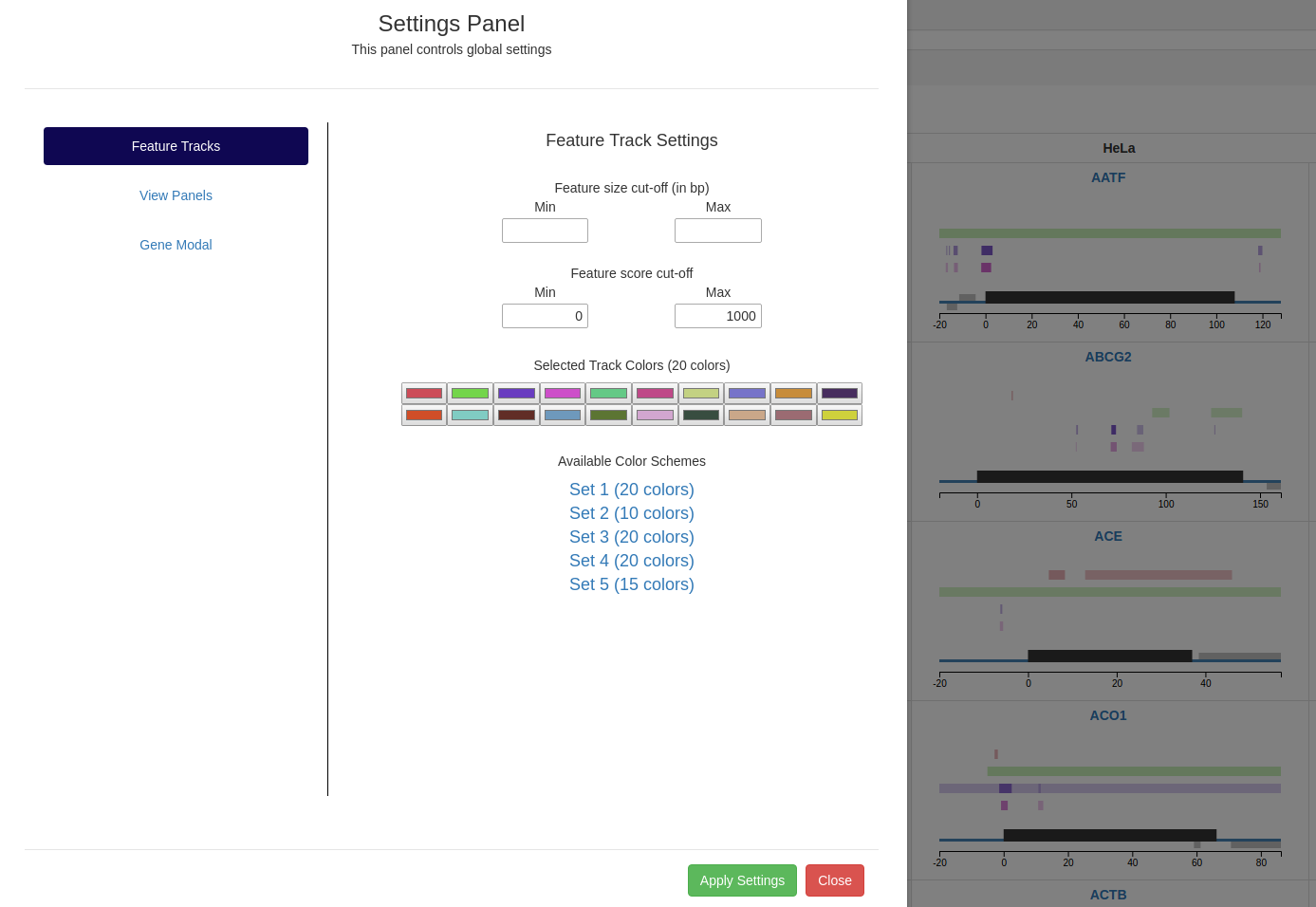
Feature track settings can be changed to define the quality of the peaks to be displayed (based on feature size and/or score). The user can provide cut-offs to ensure that only peaks meeting the selected criteria are displayed. The color of each of the feature tracks can be selected from 5 color schemes.
C-State Tutorial 11
Settings panel showing options to change feature track attributes


View Panels

Feature bar attributes (height, color) can be defined by the user. By default, exons are not displayed in the main view gene panels but they can be set for display here, along with neighboring genes. The range (default is 5th and 95th percentile) and color palette (default grayscale) used to represent the gene expression level can be customized.
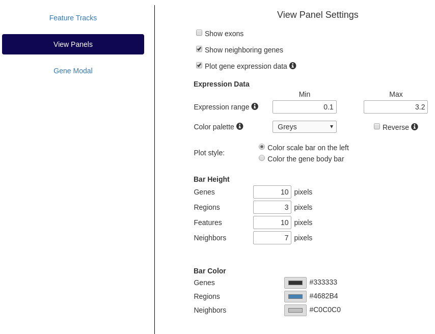
C-State Tutorial 12
Settings panel showing options to change view panel attributes


Gene Modal

Similar settings as in the main view are available here. These can be changed independently or linked to the settings in the main view.
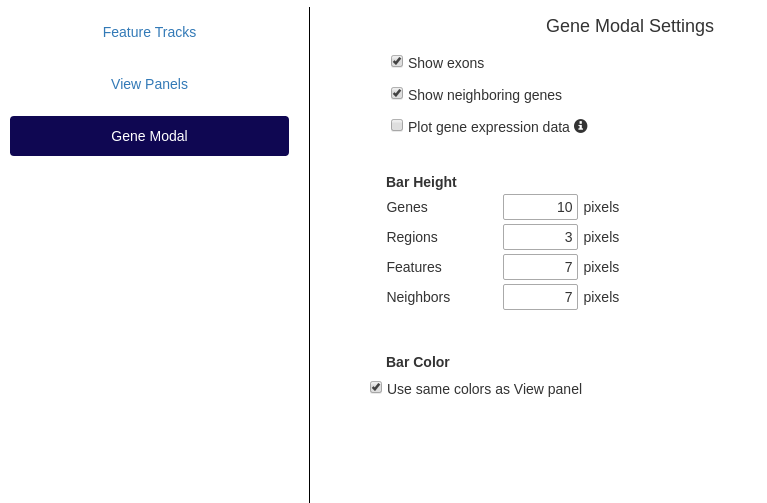
C-State Tutorial 13
Settings panel showing options to change gene modal attributes


Default Colors for C-State

Component Color Hex Value RGB Value
Gene Bar Black 333333 51,51,51 (Hue = 0)
Region Bar Steel Blue 4682B4 70,130,180
Neighbors Silver C0C0C0 192,192,192


Use Cases


Overview of datasets


Addressing biologically relevant questions often involves analyzing sets of genes belonging to particular pathways or regulating distinct cellular processes. However, extracting chromatin peak information of selected genes of interest from genome-wide datasets is a cumbersome task. The following use cases demonstrate the utility of C-State in the analysis of 16 epigenetic (4 epigenetic marks across 4 different cell types) and 4 RNA-Seq datasets from the ENCODE project. We have focussed on data from multiple human cell lines – K562, HeLa, and GM12878 – for comparison with H1 embryonic stem cells (H1-hESC) to examine changes in histone modification profiles. Whole genome ChIP-seq datasets are downloaded for H3K4me3, H3K9ac (associated with gene activation), H3K36me3 (active transcription) and H3K27me3 (repression). These datasets (see sample format) are loaded directly into C-State as feature files (Tutorial). The FPKM values of all genes derived from RNA-Seq datasets of these cell types are loaded as expression data files (see sample format). Gene expression pattern along with associated histone marks are analyzed across a selected set of 330 target genes and 20 KB of their flanking upstream and downstream regions.

Read More...

To identify enrichment patterns at a selected subset of genes in these differentiated versus pluripotent cell states, we created a list of 'stemness' genes potentially important for regulating the ES cell state from published datasets analyzing the hESC transcriptome (Bhattacharya et al., 2004) and pluripotency factor bound gene networks in hESCs (Boyer et al., 2005). A subset of 330 genes, shortlisted based on their change in expression profile upon ESC differentiation, is used here for comparative analysis.


Cell-type specific epigenetic pattern search


The chained filtering application of C-State (Filters panel) allows identification of genes bearing complex cell type specific epigenetic patterns as exemplified by the following searches

  1. Search for bivalent promoters in ESCs
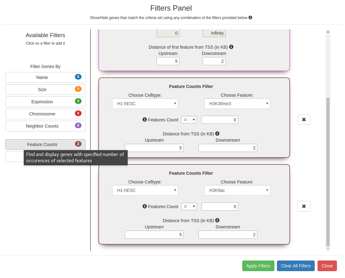
    Genes that have bivalent promoters (marked with both H3K27me3 and H3K4me3 within -5KB to +2KB of TSS) in ESCs can be identified using the "Feature Overlaps" Filter (image below on the left) chained to a couple of "Feature Counts" Filters set for the absence of the other marks (image below on the right).

    Use Case 1A
    Use Case 1B

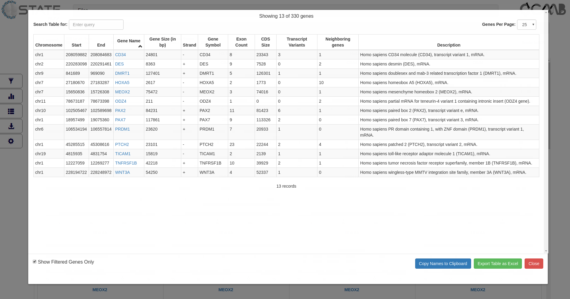
    This returns just 13 (of 330) genes. Their individual gene modals can be examined from the View accordion or a list of details obtained from the Tables panel ("Show Filtered Genes only" box checked). The bivalent gene names can also be directly copied to the clipboard for use in other applications.

    Use Case 1C

    Note: The images of all the bivalent genes and their individual modals, summary of applied filters, tabular list and plots can be saved.

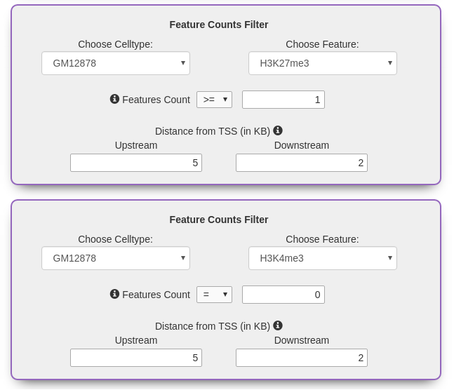
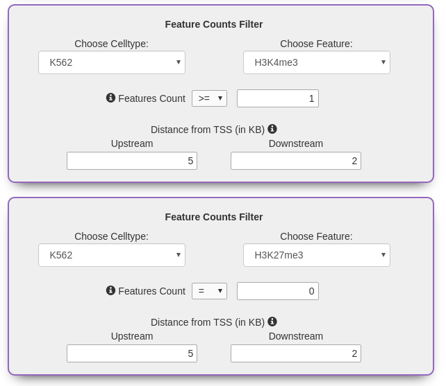
    To further identify genes where the promoter bivalents resolve into a repressed chromatin state in one cell type (GM12878, left image below) and an actively marked one in another (K562, right image below), simply add the appropriate filters to the chain.

    Use Case 1D
    Use Case 1E

    Applying this chain of 7 filters returns the muscle specific gene Desmin (DES), which has a bivalently marked promoter in ESCs that resolves into distinct chromatin states in other cell types.

    Use Case 1F

    Note: Peak score cutoffs can be applied from the Settings panel to restrict the search to features with a good score.


  2. Active Transcription in ESCs
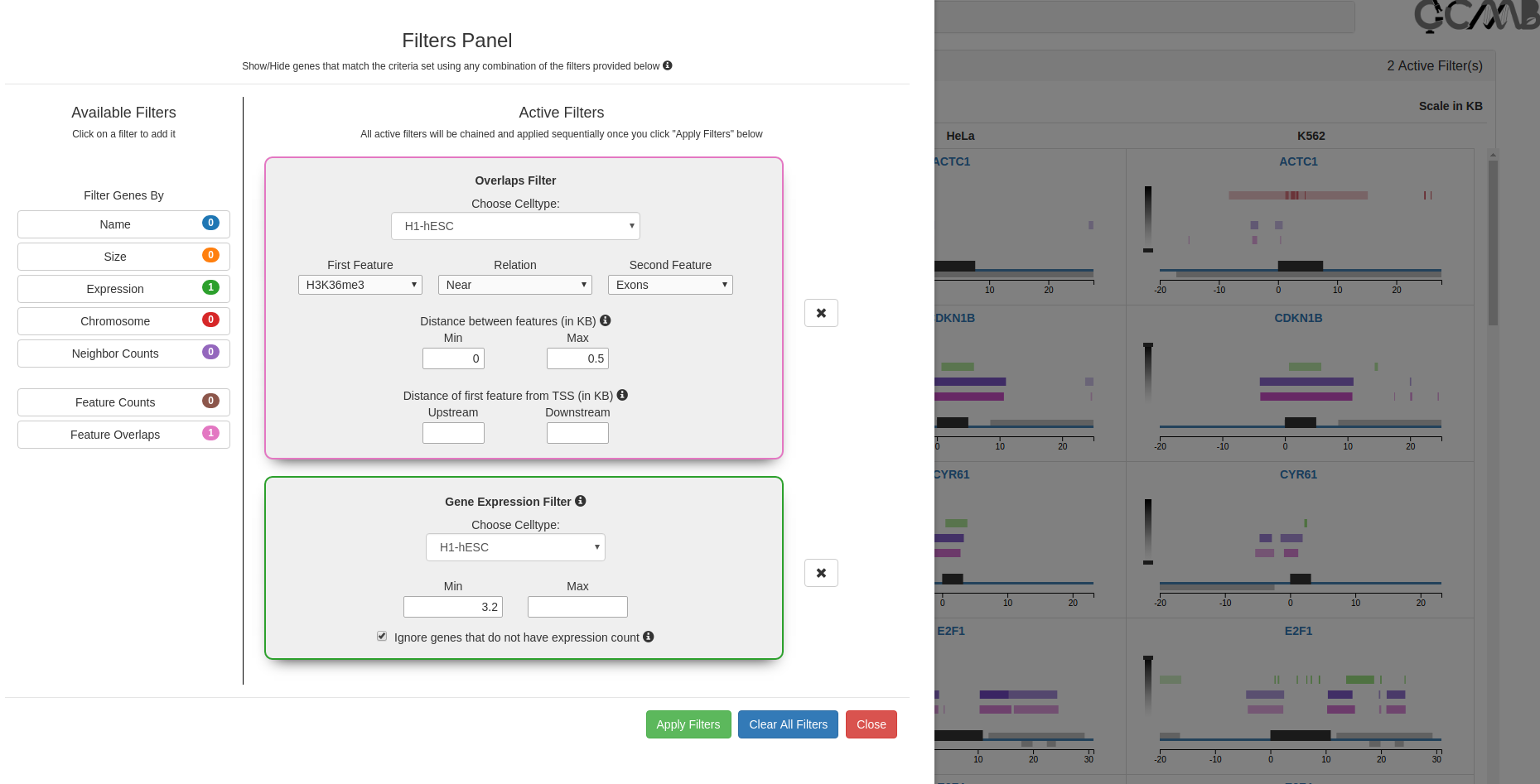
    Genes that are H3K36me3 enriched within 500 bp near exons in ESCs, indicative of active transcription, can be identified using "Feature Overlaps" Filter set for a maximum distance of 0.5 KB between a H3K36me3 peak and an exon.

    The filter returns 97 genes that match the above criteria. To further identify genes with high transcript levels, add an "Expression" filter to the chain. Set the cell type as H1-hESC, and set the minimum expression value to 3.2 (95th percentile of the loaded datasets, as depicted by the legend in the main view). This return a list of 19 genes. Analyzing these genes using the Average Feature Profile plots shows that they are generally devoid of H3K27me3 mark at their promoter regions. This indicates that the maximal gene expression in H1-hESC cells is dependent on both the presence of H3K36me3 at exons and the absence of H3K27me3 at the promoters.

    Use Case 2A


  3. Analyze Gene Families
    Compare the status of the paired box (PAX) family of transcription factors using "Name" Filter with "Match beginning only" checkbox ticked.

    Use Case 3A

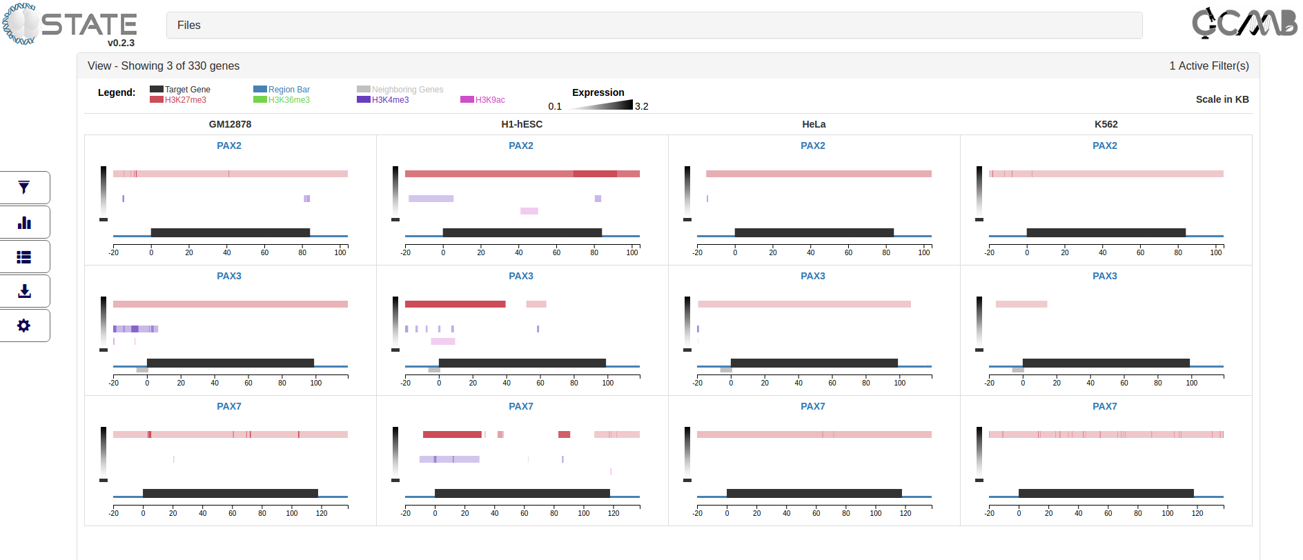
    PAX genes code for developmentally important tissue specific transcription factors needed for lineage specification. The 3 PAX genes returned by the filter show a different epigenetic profile at the TSS in ESCs compared to the differentiated cell lines (figure of View accordion below). In ESCs alone, they appear to be actively (H3K9ac) or bivalently marked (H3K4me3/H3K27me3) while the other cell types are associated with the repressive (H3K27me3) mark.

    Use Case 3B


Features distribution


Analyze global peak trends across TSS

The distribution of enriched peaks averaged across all genes can be viewed in the context of their position with respect to the gene body (TSS to TES) using the Average Feature Profile plot (Plots and Analysis panel). For the current test data of 330 genes, the plots indicate an enrichment of H3K27me3 around the TSS in ESCs but not in other cell types. The distribution of other marks, however, remains the same across all cell types. This suggests that, along with the active marks, these genes are also marked with the repressive histone mark at the TSS specifically in ESCs.

Use Case Analysis 1

Selecting the option to display TSS only (with 20KB flanks) allows investigating this pattern more closely; Filtering the genes for bivalently marked promoters in ESCs reveals a bimodal distribution of H3K27me3 peaks around the TSS - a pattern unique to ESCs.

Use Case Analysis 2


Sort and view genes by attributes


Search for non-coding genes using the Tables panel

The table view lists information in multiple columns for the genes in the gene list. Sorting for CDS size arranges the genes in ascending order of CDS size. As shown below, the first 10 genes have a CDS size of 0. These may be non coding genes and the gene modals for these can directly be opened (click on the gene name in the table) to view the peak data for this subset across cell types.

Use Case Analysis 2

This list of non-coding genes can be either exported to an Excel file, or the gene names can be copied to clipboard using the buttons on the bottom right.


Data sharing platform


C-State can also serve as a simple way to share data and basic analysis of NGS datasets. Following visualization and analysis, the user can save their settings and download the json file of the session from the Downloads panel. This C-State file can then be shared or mailed to their collaborators without needing to share the raw data or any other files. The json file simply needs to be uploaded as Previous Plot Data file into C-State and retains full functionality for visualization and downstream analysis at the other end.


In this section, we have demonstrated some of the obvious use cases of C-State. Users can also visualize other datasets such as different experimental conditions/treatments, cancerous vs normal tissues, transcription factor and other protein binding sites, genomic features such as restriction sites, CpG islands, DNaseI hyper-sensitive sites etc.


FAQs


C-State can be directly launched and run from this website using the "Launch C-State" button (Home). This is the recommended way to use C-State, as this link will always point to the latest stable version. C-State can also be downloaded as a zip file using the "Download C-State" button for local usage (for example to host on an internal server, or to use it on a system that is never online).

C-State is a 100% client-side app. This means that once the necessary data is loaded it can run independently, without the need of a working internet connection. However, processing new files and loading example data requires internet, as C-State needs to access the necessary files from our server. Once "View data" is clicked, or if you are starting with previous C-State data, or if you are using the downloaded version, C-State is fully functional even without an internet connection.

Note: The recommended way to use C-State is via the 'Launch C-State' button at the top of this page. Local installation is only needed when C-State is to be hosted on an internal network or a system not connected to the internet. To host C-State locally, follow the steps below. Some technical proficiency is expected.

As web browsers do not have permission to access the local filesystem, C-State needs to be hosted as a static server so that it can access its internal files.

To host C-State:

  1. Extract the zip file
  2. Open a Terminal/Command Prompt window in the extracted folder:

    Windows: Open the C-State folder, go to the explorer bar on the top, type "cmd" and press Enter

    Mac: Open a Terminal window (either from Utilities, or by searching in Finder). To browse to the C-State folder, type cd and drag-drop the C-State folder into the Terminal window. You should now see the path of C-State folder pasted in the Terminal. Press Enter to navigate to that directory in Terminal

    Linux users should know their stuff :)

  3. Host a static server using one of the following ways:

    Python 2.x:
    python –m SimpleHTTPServer

    Python 3.x:
    python –m http.server

    PHP:
    php –S localhost:8000

    Node.js:
    npm install -g http-server # install dependency
    http-server -p 8000

Linux and MacOS installations come with Python preinstalled. You can check your Python version using the command python –V and use the appropriate command as listed above.

For a comprehensive list of ways to host static servers, you can check this page.

Once the server is hosted, you can access C-State by opening your browser and going to http://localhost:8000.


Loading data of 330 genes, 4 histone marks and 6 cell types (Human hg19) has a peak usage of 1.1GB RAM, while loading 5000 genes, 4 histone marks, 2 cell types (Mouse mm9) uses 4GB RAM.

The following table lists the features of C-State as compared to other popular genome browsers.

Feature UCSC IGV WashU JBrowse CHROMATRA CisGenome EpiViz visPIG
Simultaneous display of multiple user-specified loci
Multiple feature tracks
Concomitant display of gene expression data
Comparison of user-generated and published datasets
Versatile filters to allow selection of user defined patterns
Interactive plotting 5
Modular and extensible
OS agnostic NA3
Programming knowledge not required
Prior dependencies not required NA 1 NA
Runs locally 2 4
Open source license

- Feature available
- Feature unavaible
NA - Not applicable

Foot notes:
1 – Needs Java Run Time, which may not be preinstalled on some systems
2 – If using the JBrowse Desktop version
3 – Runs as a plugin for Galaxy Portal
4 – If Galaxy is installed as a local instance
5 – Plotting feature could not be tested on our data

Note: ChAsE is a recently published tool for interactive visualization of input regions. As opposed to C-State's gene-centric approach, ChAsE enables comparative analysis of epigenomic datasets via k-means clustering and heat maps.


If the identifiers provided in the gene list file map to more than one isoform, C-State uses the largest isoform. To view specific isoforms of a gene, use transcript-specific IDs (for example, UCSC knownGene ID or ENSEMBL transcript IDs).

Currently, C-State supports the following genome builds:

  • hg38 (Human)
  • hg19 (Human)
  • mm10 (Mouse)
  • mm9 (Mouse)
  • rn6 (Rat)
  • rn5 (Rat)
  • galGal4 (Chicken)
  • danRer10 (Zebrafish)
  • dm6 (Drosophila)
  • dm3 (Drosophila)
  • ce11 (Worm (C. elegans))
  • ce10 (Worm (C. elegans))
  • sacCer3 (Yeast)
  • sacCer2 (Yeast)


No. As C-State works with coordinate based information, any annotation or feature that can be described in BED format (e.g. exons, CpG islands, restriction sites, SNPs etc.) can be plotted as data tracks.


Any numerical value which indicates the relative expression level of a gene is accepted by C-State. For example, they could be raw read counts, RPKM, FPKM, CPM or TPM values from RNA-Seq experiments, or Normalized Log Ratios from microarray experiments. However, as expression values are compared across genes and cell types, we recommend using normalized values such as FPKM or CPM.


C-State was primarily designed for analysis and filtering of genes based on their chromatin signatures. Hence, it is fully functional even if no expression data is loaded. In fact, C-State can also handle data inputs where the expression of only some of the target genes is loaded.


C-State supports UCSC genome browser-type shading of features based on scores, which are in a range of 1 to 1000 (1000 being the best and 1 being the least score). Ensure that your feature scores are also in the same range. You can also disable the shading feature altogether by either removing your score information or by using a score of 0 for all features in your input files. In such cases, the score is displayed as 'NA' on mouse-hover.


C-State runs in all browsers which support HTML5 and ES2015 (the 2015 version of JavaScript). If you have updated your browser in the last one year, then your browser can run C-State. We have extensively developed and tested it in Google Chrome and hence recommend it, however we had no issues running it in latest versions of Mozilla Firefox and Microsoft Edge.


There are no arbitrary limitations imposed by C-State with respect to the number of genes, cell types or features to be plotted. However, the actual number that can be realistically plotted at one go is limited primarily by the total available RAM in the system. Also, plotting too many cell types or conditions on a single page (more than 8 in our opinion) can be aesthetically constraining.


This happens if some of the gene identifiers specified did not match any identifier in the genome (because of aliases etc.). C-State alerts the user in case some IDs could not be mapped. If none of the identifiers could be mapped, it mostly indicates that the chosen identifier type is wrong. C-State does not let the user proceed to next steps unless at least one gene identifier is successfully mapped.


This is a browser setting that can easily changed. For example, on Google Chrome, you can go to Settings -> Show Advanced Settings -> Downloads, and check the box that says "Ask where to save each file before downloading". On Mozilla Firefox, you can change this from Preferences -> General -> Downloads and select the radio button that says "Always ask me where to save files"


If C-State encounters an error in processing files, it flashes an alert. The timer spinning endlessly could indicate a system memory issue. In such a case close any other applications and reload C-State.


Contact Us


For queries or suggestions please contact:


To Cite C-State:

C-State: an interactive web app for simultaneous multi-gene visualization and comparative epigenetic pattern search
Divya Tej Sowpati, Surabhi Srivastava, Jyotsna Dhawan, Rakesh Mishra
BMC Bioinformatics 2017 18(Suppl 10):392
doi: 10.1186/s12859-017-1786-6

Last updated on 27th September, 2017.

Website developed by Saketh Saxena; Maintained and managed by Divya Tej Sowpati.

The intial prototype for C-State v0.1 was created by Saurabh Gaur.